R Studio Lavan Download Error
Purpose
This seminar will show you how to perform a confirmatory factor analysis using lavaan in the R statistical programming language. Its emphasis is on understanding the concepts of CFA and interpreting the output rather than a thorough mathematical treatment or a comprehensive list of syntax options in lavaan. For exploratory factor analysis (EFA), please refer to A Practical Introduction to Factor Analysis: Exploratory Factor Analysis. A rudimentary knowledge of linear regression is required to understand some of the material in this seminar.
This seminar is the first in a three-part series on latent variable modeling. The second seminar goes over a broader range of observed and latent variable models. In this first seminar, all variables are presumed to be $y$-side variables and the direction of the arrows are unconventional (pointing to the left). Traditionally, CFA models should be $x$-side variables with parameters $\xi$ for the latent factor and $\delta$ for the observed residuals. Since $y$-side notation is more common in the literature, we use $\eta$ and $\epsilon$ for the respective factor and observed residual parameters. However, in the second seminar we necessitate distinguishing between $x$-side and $y$-side variables for instructional purposes.
- Introduction to Structural Equation Modeling (SEM) in R with lavaan.
The third seminar goes over intermediate topics in CFA including latent growth modeling and measurement invariance.
- Latent Growth Models (LGM) and Measurement Invariance with R in lavaan
Outline
Proceed through the seminar in order or click on the hyperlinks below to go to a particular section:
- Introduction
- Motivating example SPSS Anxiety Questionairre
- The factor analysis model
- The model-implied covariance matrix
- The path diagram
- One Factor Confirmatory Factor Analysis
- Known values, parameters, and degrees of freedom
- Three-item (one) factor analysis
- Identification of a three-item one factor CFA
- Running a one-factor CFA in lavaan
- (Optional) How to manually obtain the standardized solution
- (Optional) Degrees of freedom with means
- One factor CFA with two items
- One factor CFA with more than three items (SAQ-8)
- Model Fit Statistics
- Model chi-square
- A note on sample size
- (Optional) Model test of the baseline or null model
- Incremental versus absolute fit index
- CFI (Comparative Fit Index)
- TLI (Tucker Lewis Index)
- RMSEA
- Two Factor Confirmatory Factor Analysis
- Uncorrelated factors
- Correlated factors
- Second-Order CFA
- (Optional) Warning message with second-order CFA
- (Optional) Obtaining the parameter table
- Conclusion
- Appendix
- References
Back to Launch Page
Requirements
Before beginning the seminar, please make sure you have R and RStudio installed.
Please also make sure to have the following R packages installed, and if not, run these commands in R (RStudio).
install.packages("foreign", dependencies=TRUE) install.packages("lavaan", dependencies=TRUE) Once you've installed the packages, you can load them via the following
library(foreign) library(lavaan)
Download files here
You may download the complete R code here: cfa.r
After clicking on the link, you can copy and paste the entire code into R or RStudio.
PowerPoint slides for the seminar given on 05/17/2021 are here: PowerPoint Slides for Intro to CFA
The corresponding code for the exercises are included here: R Code for Intro to CFA (Supplementary Exercises)
Introduction
Factor analysis can be divided into two main types, exploratory and confirmatory. Exploratory factor analysis, also known as EFA, as the name suggests is an exploratory tool to understand the underlying psychometric properties of an unknown scale. Confirmatory factor analysis borrows many of the same concepts from exploratory factor analysis except that instead of letting the data tell us the factor structure, we pre-determine the factor structure and verify the psychometric structure of a previously developed scale. More recent work by Asparouhov and Muthén (2009) blurs the boundaries between EFA and CFA, but traditionally the two methods have been distinct. EFA has a longer historical precedence, dating back to the era of Spearman (1904) whereas CFA became more popular after a breakthrough in both computing technology and an estimation method developed by Jöreskog (1969). This distinction shows up in software as well. For example, EFA is available in SPSS FACTOR, SAS PROC FACTOR and Stata's factor. However, in SPSS a separate program called Amos is needed to run CFA, along with other packages such as Mplus, EQS, SAS PROC CALIS, Stata's sem and more recently, R's lavaan. Since the focus of this seminar is CFA and R, we will focus on lavaan.
In this seminar, we will understand the concepts of CFA through the lens of a statistical analyst tasked to explore the psychometric properties of a newly proposed 8-item SPSS Anxiety Questionnaire. Due to budget constraints, the lab uses the freely available R statistical programming language, and lavaan as the CFA and structural equation modeling (SEM) package of choice. We will understand concepts such as the factor analysis model, basic lavaan syntax, model parameters, identification and model fit statistics. These concepts are crucial to deciding how many items to use per factor, as well how to successfully fit a one-factor, two-factor and second-order factor analysis. By the end of this training, you should be able to understand enough of these concepts to run your own confirmatory factor analysis in lavaan.
Motivating example: SPSS Anxiety Questionnaire (SAQ-8)
Suppose you are tasked with evaluating a hypothetical but real world example of a questionnaire which Andy Field terms the SPSS Anxiety Questionnaire (SAQ). The first eight items consist of the following (note the actual items have been modified slightly from the original data set):
- Statistics makes me cry
- My friends will think I'm stupid for not being able to cope with SPSS
- Standard deviations excite me
- I dream that Pearson is attacking me with correlation coefficients
- I don't understand statistics
- I have little experience with computers
- All computers hate me
- I have never been good at mathematics
Throughout the seminar we will use the terms items and indicators interchangeably, with the latter emphasizing the relationship of these items to a latent variable. Just as in our exploratory factor analysis our Principal Investigator would like to evaluate the psychometric properties of our proposed 8-item SPSS Anxiety Questionnaire "SAQ-8", proposed as a shortened version of the original SAQ in order to shorten the time commitment for participants while maintaining internal consistency and validity. The data collectors have collected 2,571 subjects so far and uploaded the SPSS file to the IDRE server. The SPSS file can be download through the following link: SAQ.sav. Even though this is an SPSS file, R can translate this file directly to an R object through the function read.spss via the library foreign. The option to.data.frame ensures the data imported is a data frame and not an R list, and use.value.labels = FALSE converts categorical variables to numeric values rather than factors. This is done because we want to run covariances on the items which is not possible with factor variables.
dat <- read.spss("https://stats.idre.ucla.edu/wp-content/uploads/2018/05/SAQ.sav", to.data.frame=TRUE, use.value.labels = FALSE) Now that we have imported the data set, the first step besides looking at the data itself is to look a the correlation table of all 8 variables. The function cor specifies a the correlation and round with the option 2 specifies that we want to round the numbers to the second digit.
> round(cor(dat[,1:8]),2) q01 q02 q03 q04 q05 q06 q07 q08 q01 1.00 -0.10 -0.34 0.44 0.40 0.22 0.31 0.33 q02 -0.10 1.00 0.32 -0.11 -0.12 -0.07 -0.16 -0.05 q03 -0.34 0.32 1.00 -0.38 -0.31 -0.23 -0.38 -0.26 q04 0.44 -0.11 -0.38 1.00 0.40 0.28 0.41 0.35 q05 0.40 -0.12 -0.31 0.40 1.00 0.26 0.34 0.27 q06 0.22 -0.07 -0.23 0.28 0.26 1.00 0.51 0.22 q07 0.31 -0.16 -0.38 0.41 0.34 0.51 1.00 0.30 q08 0.33 -0.05 -0.26 0.35 0.27 0.22 0.30 1.00
In a typical variance-covariance matrix, the diagonals constitute the variances of the item and the off-diagonals the covariances. The interpretation of the correlation table are the standardized covariances between a pair of items, equivalent to running covariances on the Z-scores of each item. In a correlation table, the diagonal elements are always one because an item is always perfectly correlated with itself. Recall that the magnitude of a correlation $|r|$ is determined by the absolute value of the correlation. From this table we can see that most items have magnitudes ranging from $|r|=0.38$ for Items 3 and 7 to $|r|=0.51$ for Items 6 and 7. Notice that the correlations in the upper right triangle (italicized) are the same as those in the lower right triangle, meaning the correlation for Items 6 and 7 is the same as the correlation for Items 7 and 6. This property is known as symmetry and will be important later on.
In psychology and the social sciences, the magnitude of a correlation above 0.30 is considered a medium effect size. Due to relatively high correlations among many of the items, this would be a good candidate for factor analysis. The goal of factor analysis is to model the interrelationships between many items with fewer unobserved or latent variables. Before we move on, let's understand the confirmatory factor analysis model.
The factor analysis model
The factor analysis or measurement model is essentially a linear regression model where the main predictor, the factor, is latent or unobserved. For a single subject, the simple linear regression equation is defined as:
$$y = b_0 + b_1 x + \epsilon$$
where \(b_0\) is the intercept and \(b_1\) is the coefficient and \(x\) is an observed predictor. Similarly, for a single item, the factor analysis model is:
$$y_{1} = \tau_1 + \lambda_1 \eta + \epsilon_{1} $$
where is the $\tau_1$ intercept of the first item and $\lambda_1$ is the loading or regression weight of the first factor on the first item, and \(\epsilon_1\) is the residual for the first item. There are three main differences between the factor analysis model and linear regression:
- Factor analysis outcomes are items not observations, so $y_1$ indicates the first item.
- Factor analysis is a multivariate model there are as many outcomes per subject as there are items. In a linear regression, there is only one outcome per subject.
- The predictor or factor, \(\eta\) ("eta"), is unobserved whereas in a linear regression the predictors are observed.
We can represent this multivariate model (i.e., multiple outcomes, items, or indicators) as a matrix equation:
$$ \begin{pmatrix} y_{1} \\ y_{2} \\ y_{3} \end{pmatrix} = \begin{pmatrix} \tau_1 \\ \tau_2 \\ \tau_3 \end{pmatrix} + \begin{pmatrix} \lambda_{1} \\ \lambda_{2} \\ \lambda_{3} \end{pmatrix} \begin{pmatrix} \eta_{1} \end{pmatrix} + \begin{pmatrix} \epsilon_{1}\\ \epsilon_{2} \\ \epsilon_{3} \end{pmatrix} $$
The equivalent three sets of equations are written as: $$ \begin{matrix} y_1 = \tau_1 + \lambda_{1}\eta_{1} + \epsilon_{1} \\ y_2 = \tau_2 + \lambda_{2}\eta_{1} + \epsilon_{2} \\ y_3 = \tau_3 + \lambda_{3}\eta_{1} + \epsilon_{3} \end{matrix} $$
Let's define each of the terms in the model
- $\tau$ ("tau") the item intercepts or means
- $\lambda$ ("lambda") the loadings, which can be interpreted as the correlation of the item with the factor
- $\eta$ ("eta"), the latent predictor of the items, i.e. the factor (SPSS Anxiety)
- $\epsilon$ ("epsilon") the residuals of the factor model, what's left over after accounting for the factor (what SPSS Anxiety does not explain)
The index refers to the item number. So for example $\tau_1$ means the intercept of the first item, $\lambda_2$ is the loading of the second item with the factor and $\epsilon_{3}$ is the residual of the third item, after accounting for the factor.
The model-implied covariance matrix
Historically, factor analysis is used to answer the question, how much common variance is shared among the items. This variance-covariance matrix can be described using the model-implied covariance matrix $\Sigma(\Theta)$. Note that this is in contrast to theobserved population covariance matrix $\Sigma$ which comes only from the data. The formula for the model-implied covariance matrix is:
$$ \Sigma(\theta) = \mathbf{\Lambda \Psi \Lambda'} + \Theta_{\epsilon} $$
The following describes eachparameter, defined as a term in the model to be estimated:
- $\mathbf{\Lambda}$ ("lambda") factor loading matrix (consisting of the same $\lambda$'s from the measurement model)
- $\mathbf{\Psi}$ ("psi") variance-covariance matrix of the latent factors (i.e., variance of $\eta$; for one factor, it is a scalar)
- $\mathbf{\Theta_{\epsilon}}$ ("theta-epsilon") variance-covariance matrix of the residuals
The dimensions of this matrix correspond to the same as that of the observed covariance matrix $\Sigma$, for three items it is $3 \times 3$. Recall that the model covariance matrix can be defined by the following:
In the three item one-factor case,
$$ \Sigma(\theta) = \begin{pmatrix} \lambda_{1} \\ \lambda_{2} \\ \lambda_{3} \end{pmatrix} \begin{pmatrix} \psi_{11} \end{pmatrix} \begin{pmatrix} \lambda_{1} & \lambda_{2} & \lambda_{3} \end{pmatrix} + \begin{pmatrix} \theta_{11} & \theta_{12} & \theta_{13} \\ \theta_{21} & \theta_{22} & \theta_{23} \\ \theta_{31} & \theta_{32} & \theta_{33} \\ \end{pmatrix} $$
Note that the loadings $\lambda$ are the same parameters shared between the measurement model and the model-implied covariance model. This means the only new parameters involve the $\Psi$ and the $\Theta_{\epsilon}$ which are the covariance matrices of the latent factors and residual errors respectively. Why do we care so much about the variance-covariance matrix of the items? Because the basic assumption of factor analysis is that for a collection of observed variables there are a set of underlying factors (smaller than the observed variables, i.e., the \(\eta\)s), that can explain the interrelationships among those variables. These interrelationships are measured by the covariances.
The path diagram
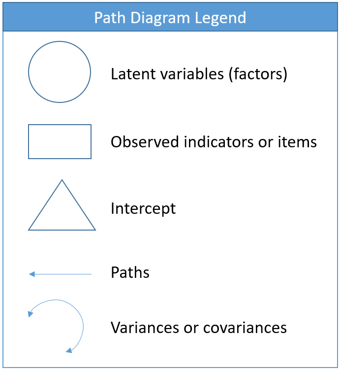
Equations can be intimidating. The path diagram can assist us in understanding our CFA model because it is a symbolic one-to-one visualization of the measurement model and the model-implied covariance. Before we present the actual path diagram, the table below defines the symbols we will be using. Circles represent latent variables, squares represent observed indicators, triangles represent intercept or means, one-way arrows represent paths and two-way arrows represent either variances or covariances.
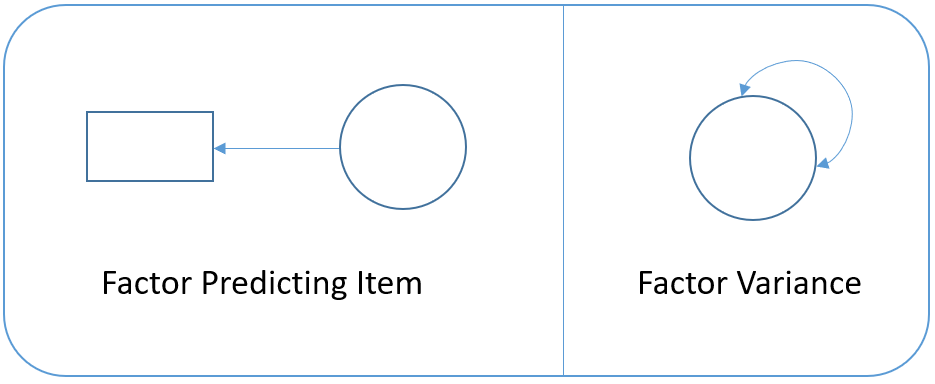
For example in the figure below, the diagram on the left depicts the regression of a factor on an item (essentially a measurement model) and the diagram on the right depicts the variance of the factor (a two-way arrow pointing to an latent variable).
In the path diagram below, all measurement model parameters are color-coded in green and all model-implied covariance parameters are coded in blue. As a general rule only paths ($\lambda,\tau$) and bidirectional arrows ($\psi$) are estimated, not circles or squares (i.e., $y, \epsilon, \eta$). Then the only green paths are $\lambda,\tau$, and among the blue, again $\lambda$ is estimated, as well as $\theta$ and $\psi$. However, the $\lambda$ is the same across measurement and covariance models so we do not need to estimate them twice. Traditionally, the $\tau$ is not estimated, which means that all the parameters we need can come directly from the covariance model.
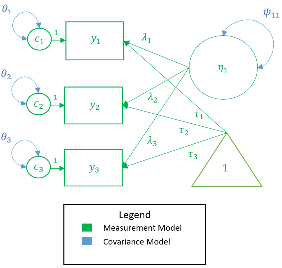
In the model-implied covariance, we assume that the residuals are independent which means that for example $\theta_{21}$, the covariance between the second and first residual, is set to to zero. As such the only covariance terms to be estimated are $\psi_{11}$ which is the variance of the factor, and $\theta_{11}, \theta_{22}$ and $\theta_{33}$ which are the variances of the residuals (assuming hetereoskedastic variances). As an exercise, see if you can map the path diagram above to the following regression equations:
$$ \begin{matrix} y_1 = \tau_1 + \lambda_{1}\eta_{1} + \epsilon_{1} \\ y_2 = \tau_2 + \lambda_{2}\eta_{1} + \epsilon_{2} \\ y_3 = \tau_3 + \lambda_{3}\eta_{1} + \epsilon_{3} \end{matrix} $$
$$ \Sigma(\theta) = \begin{pmatrix} \lambda_{1} \\ \lambda_{2} \\ \lambda_{3} \end{pmatrix} \begin{pmatrix} \psi_{11} \end{pmatrix} \begin{pmatrix} \lambda_{1} & \lambda_{2} & \lambda_{3} \end{pmatrix} + \begin{pmatrix} \theta_{11} & 0 & 0 \\ 0 & \theta_{22} & 0 \\ 0 & 0 & \theta_{33} \\ \end{pmatrix} $$
The path diagram and the equations quickly inform us of the parameters coming either from the measurement model or model-implied covariance; and knowing how to count parameters is an essential. Traditionally, we disregard the parameters in the measurement model model (i.e., $\tau$), and here focus on the parameters from the covariance model. See if you can count the number of parameters from the equations or path diagram above. As a data analyst, knowing how to count parameters is surprisingly crucial in understanding an essential CFA concept called identification.
Answer
There are three loadings, $\lambda_1, \lambda_2, \lambda_3$, one factor variance, $\psi_{11}$ and three residual variances $\theta_1, \theta_2, \theta_3$. However, we only have six known values from the observed covariance matrix.
One factor confirmatory factor analysis
The most fundamental model in CFA is the one factor model, which will assume that the covariance among items is due to a single common factor. Suppose the Principal Investigator is interested in testing the assumption that the first items in the SAQ-8 is a reliable estimate measure of SPSS Anxiety. The eight items are observed indicators of the latent or unobserved construct which the PI calls SPSS Anxiety. The items are the fundamental elements in a CFA and the covariances between the items forms the the fundamental component in CFA. The observed population covariance matrix $\Sigma$ is a matrix of bivariate covariances that determines how many total parameters can be estimated in the model. The model implied matrix $\Sigma(\theta)$ has the same dimensions as $\Sigma$. Recall that the model implied covariance matrix is defined as
$$ \Sigma(\theta) = Cov(\mathbf{y}) = {\Lambda} \Psi \mathbf{\Lambda}' + \Theta_{\epsilon} $$
This means that $\theta$ is composed of the parameters $\Lambda, \Psi, \Theta_{\epsilon}$, which correspond to the loadings, the covariances of the latent variables and the covariance of the residual errors. Notice that the observed indicators $y$ are not part of the set of parameters, but are instead used to estimate the parameters. As a simple analogy, suppose you have a data set with observed outcomes $y = 13, 14, 15$, then the mean parameter, $\mu$, the estimate of this parameter is called "mu-hat" denoted $\hat{\mu}=\bar{y}=\frac{1}{n}\sum y_i$. Here $\bar{y}= (13+14+15)/3=14$. Similarly, in CFA the items are used to estimate all the parameters the model-implied covariance, which correspond to $\hat{\Lambda}, \hat{\Psi}, \hat{\Theta_{\epsilon}}$, the carrot or hat symbol emphasizing that these parameters are estimated. In an ideal world you would have an unlimited number of items to estimate each parameter, however in the real world there are restrictions to the total number of parameters you can use. These restrictions are known as identification. To understand this concept, we will talk about fixed versus free parameters in a CFA.
Known values, parameters, and degrees of freedom
The concept of a fixed or free parameter is essential in CFA. The total number of parameters in a CFA model is determined by the number of known values in your population variance-covariance matrix $\Sigma$, given by the formula $p(p+1)/2$ where $p$ is the number of items in your survey. Suppose the principal investigator thinks that the third, fourth and fifth items of the SAQ are the observed indicators of SPSS Anxiety. To obtain the sample covariance matrix $S=\hat{\Sigma}$, which is an estimate of the population covariance matrix $\Sigma$, use the column index [,3:5], and the command cov. The function round with the option 2 specifies that we want to round the numbers to the second digit.
> round(cov(dat[,3:5]),2) q03 q04 q05 q03 1.16 -0.39 -0.32 q04 -0.39 0.90 0.37 q05 -0.32 0.37 0.90
The off-diagonal cells in $S$ correspond to bivariate sample covariances between two pairs of items; and the diagonal cells in $S$ correspond to the sample variance of each item (hence the term "variance-covariance matrix"). Item 3 has a negative relationship with Items 4 and 5 but Item 4 has a positive relationship with Item 5. Just as in the correlation matrix we calculated before, the lower triangular elements in the covariance matrix are duplicated with the upper triangular elements. For example, the covariance of Item 3 with Item 4 is -0.39, which is the same as the covariance of Item 4 and Item 3 (recall the property of symmetry). Because the covariances are duplicated, the number of free parameters in CFA is determined by the number of uniquevariances and covariances. With three items, the number of known values is $3(4)/2=6$. The known values serve as the primary restriction in terms of how manytotalparameters we can estimate. For simplicity, let's assume that the total number of parameters comeonlyfrom the model-implied covariance matrix. See the optional section Degrees of freedom with means for the more technically accurate explanation of total parameters. Given that we have 6 known values, how many (unique) total parameters do we have from the model-implied covariance matrix?
$$ \Sigma(\theta)= \begin{pmatrix} \lambda_{1} \\ \lambda_{2} \\ \lambda_{3} \end{pmatrix} \begin{pmatrix} \psi_{11} \end{pmatrix} \begin{pmatrix} \lambda_{1} & \lambda_{2} & \lambda_{3} \\ \end{pmatrix} + \begin{pmatrix} \theta_{11} & \theta_{12} & \theta_{13} \\ \theta_{21} & \theta_{22} & \theta_{23} \\ \theta_{31} & \theta_{32} & \theta_{33} \\ \end{pmatrix} $$
If we were to estimate every (unique) parameter in the model-implied covariance matrix, there would be 3 $\lambda$'s, 1 $\psi$, and 6 $\theta$'s (since by symmetry, $\theta_{12}=\theta_{21}$, $\theta_{13}=\theta_{31}$, and $\theta_{23}=\theta_{32}$) which gives you a total of 10 total parameters, but we only have 6 known values! The solution is to allow for fixed parameters which are parameters that are not estimated and pre-determined to have a specific value. We will talk more about fixed parameters when we discuss identification, but as a silly example, suppose we fix all parameters to either 1 or 0.
$$ \Sigma(\theta)= \begin{pmatrix} \lambda_{1} = 1 \\ \lambda_{2} = 1 \\ \lambda_{3} =1 \end{pmatrix} \begin{pmatrix} \psi_{11} =1 \end{pmatrix} \begin{pmatrix} \lambda_{1} =1 & \lambda_{2} = 1 & \lambda_{3}=1 \\ \end{pmatrix} + \begin{pmatrix} \theta_{11} = 1 & \theta_{12} =0 & \theta_{13} =0 \\ \theta_{21} =0 & \theta_{22} =1 & \theta_{23} =0 \\ \theta_{31} =0 & \theta_{32} =0 & \theta_{33} = 1 \\ \end{pmatrix} $$
How many total (unique) parameters have we fixed here? (Answer: 10) The number of free parametersis defined as
$$\mbox{number of free parameters} = \mbox{number of unique parameters } – \mbox{number of fixed parameters}.$$
How many free parameters have we obtained after fixing 10 (unique) parameters? (Answer: $10 – 10 = 0$). The goal is to maximize the degrees of freedom (df) which is defined as
$$\mbox{df} = \mbox{number of known values } – \mbox{ number of free parameters}$$
How many degrees of freedom do we have now? (Answer: $6 – 0 = 6$)
The example above is unrealistic because it would be pointless to have all the parameters be fixed. Instead, many models are just-identified or saturated with zero degrees of freedom. This means that the number of free parameters takes up all known values in $\Sigma$. This is commonly seen in linear regression models, and the main drawback is that we cannot assess its model fit because it supposedly is the best we can do. An under-identified model means that the number of known values is less than the number of free parameters, which is undesirable. In CFA, what we really want is an over-identified model where the number of known values is greater than the number of free parameters. Over-identified models allow us to assess model fit (to be discussed later). To summarize
- df negative, known < free (under-identified, bad)
- df = 0, known = free (just identified or saturated, neither bad nor good)
- df positive, known > free (over-identified, good)
Quiz
Before fixing the 10 unique parameters, we were under-identified. Explain why fixing $\lambda_1=1$ and setting the unique residual covariances to zero (e.g., $\theta_{12}=\theta_{21}=0$, $\theta_{13}=\theta_{31}=0$, and $\theta_{23}=\theta_{32}=0$) results in a just-identified model. Use the equations to help you.
Answer: We start with 10 total parameters in the model-implied covariance matrix. Since we fix one loading, and 3 unique residual covariances, the number of free parameters is $10-(1+3)=6$. Since we have 6 known values, our degrees of freedom is $6-6=0$, which is defined to be saturated. This is known as the marker method.
Three-item (one) factor analysis
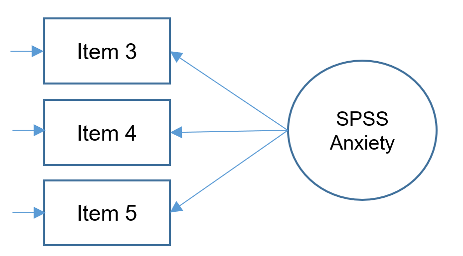
For edification purposes, let's suppose that due to budget constraints, only three items were collected from the SAQ-8. The following simplified path diagram depicts the SPSS Anxiety factor indicated by Items 3, 4 and 5 (note what's missing from the complex diagram introduced in previous sections).
Thankfully for us, we have just the right amount of items to fit a CFA because a three-item one factor CFA is just-identified, meaning it has zero degrees of freedom. Because this model is on the brink of being under-identified, it is a good model for introducing identification, which is the process of ensuring each free parameter in the CFA has a unique solution and making surer the degrees of freedom is at least zero. There are many rules for proper identification, but for the casual analyst identification helps us avoid the following message in lavaan:
lavaan WARNING: Could not compute standard errors! The information matrix could not be inverted. This may be a symptom that the model is not identified.
Identification of a three-item one factor CFA
Identification for the one factor CFA with three items is necessary due to the fact that we have seven total parameters from the model-implied covariance matrix $\Sigma(\theta)$ but only six known values from the observed population covariance matrix $\Sigma$ to work with. The total parameters include three factor loadings, three residual variances and one factor variance. The extra parameter comes from the fact that we do not observe the factor but are estimating its variance. In order to identify a factor in a CFA model with three or more items, there are two options known respectively as the marker method and the variance standardization method. The
- marker method fixes the first loading of each factor to 1,
- variance standardization method fixes the variance of each factor to 1 but freely estimates all loadings.
In matrix notation, the marker method (Option 1) can be shown as
$$ \Sigma(\theta)= \psi_{11} \begin{pmatrix} 1 \\ \lambda_{2} \\ \lambda_{3} \end{pmatrix} \begin{pmatrix} 1 & \lambda_{2} & \lambda_{3} \\ \end{pmatrix} + \begin{pmatrix} \theta_{11} & 0 & 0 \\ 0 & \theta_{22} & 0 \\ 0 & 0 & \theta_{33} \\ \end{pmatrix} $$
In matrix notation, the variance standardization method (Option 2) looks like
$$ \Sigma(\theta)= (1) \begin{pmatrix} \lambda_{1} \\ \lambda_{2} \\ \lambda_{3} \end{pmatrix} \begin{pmatrix} \lambda_{1} & \lambda_{2} & \lambda_{3} \\ \end{pmatrix} + \begin{pmatrix} \theta_{11} & 0 & 0 \\ 0 & \theta_{22} & 0 \\ 0 & 0 & \theta_{33} \\ \end{pmatrix} $$
Notice in both models that the residual covariances stay freely estimated.
Quiz
For the variance standardization method, go through the process of calculating the degrees of freedom. If we have six known values is this model just-identified, over-identified or under-identified?
Answer: We start with 10 unique parameters in the model-implied covariance matrix. Since we fix one factor variance, and 3 unique residual covariances, the number of free parameters is $10-(1+3)=6$. Since we have 6 known values, our degrees of freedom is $6-6=0$, which is defined to be saturated. This is known as the variance standardization method.
Running a one-factor CFA in lavaan
Before running our first factor analysis, let us introduce some of the most frequently used syntax in lavaan
-
~predict, used for regression of observed outcome to observed predictors -
=~indicator, used for latent variable to observed indicator in factor analysis measurement models -
~~covariance -
~1intercept or mean (e.g.,q01 ~ 1estimates the mean of variableq01) -
1*fixes parameter or loading to one -
NA*frees parameter or loading (useful to override default marker method) -
a*labels the parameter 'a', used for model constraints
Now that we are familiar with some syntax rules, let's see how we can run a one-factor CFA in lavaan with Items 3, 4 and 5 as indicators of your SPSS Anxiety factor.
#one factor three items, default marker method m1a <- ' f =~ q03 + q04 + q05' onefac3items_a <- cfa(m1a, data=dat) summary(onefac3items_a)
The first line is the model statement. Recall that =~ represents the indicator equation where the latent variable is on the left and the indicators (or observed variables) are to the right the symbol. Here we name our factor f (or SPSS Anxiety), which is indicated by q03, q04 and q05 whose names come directly from the dataset. We store the model into object m1a for Model 1A. The second line is where we specify that we want to run a confirmatory factor analysis using the cfa function, which is actually a wrapper for the lavaan function. The model to be estimatd is m1a and the dataset to be used is dat; storing the output into object onefac3items_a. Finally the third line requests textual output for onefac3items_a, listing for example the estimator used, the number of free parameters, the test statistic, estimated means, loadings and variances.
lavaan 0.6-5 ended normally after 23 iterations Estimator ML Optimization method NLMINB Number of free parameters 6 Number of observations 2571 Model Test User Model: Test statistic 0.000 Degrees of freedom 0 Parameter Estimates: Information Expected Information saturated (h1) model Structured Standard errors Standard Latent Variables: Estimate Std.Err z-value P(>|z|) f =~ q03 1.000 q04 -1.139 0.073 -15.652 0.000 q05 -0.945 0.056 -16.840 0.000 Variances: Estimate Std.Err z-value P(>|z|) .q03 0.815 0.031 26.484 0.000 .q04 0.458 0.030 15.359 0.000 .q05 0.626 0.025 24.599 0.000 f 0.340 0.031 11.034 0.000
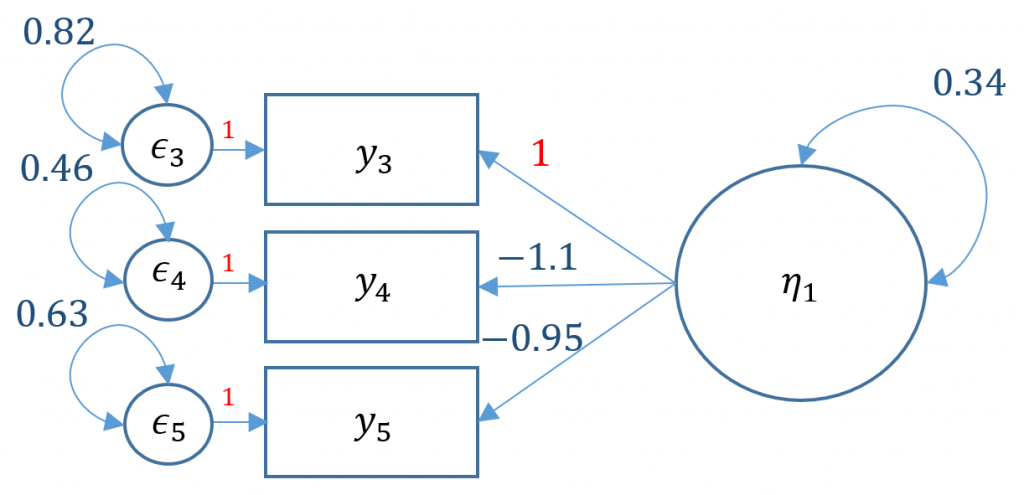
By default, lavaan chooses the marker method (Option 1) if nothing else is specified. In order to free a parameter, put NA* in front of the parameter to be freed, to fix a parameter to 1, put 1* in front of the parameter to be fixed. The syntax NA*q03 frees the loading of the first item because by default marker method fixes it to one, and f ~~ 1*f means to fix the variance of the factor to one.
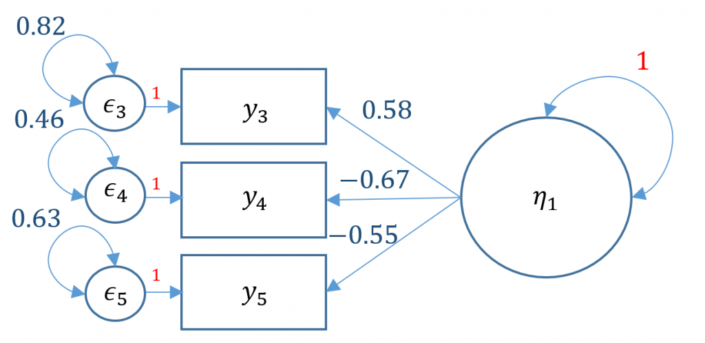
#one factor three items, variance std m1b <- ' f =~ NA*q03 + q04 + q05 f ~~ 1*f ' onefac3items_b <- cfa(m1b, data=dat) summary(onefac3items_b) <...output omitted...> Latent Variables: Estimate Std.Err z-value P(>|z|) f =~ q03 0.583 0.026 22.067 0.000 q04 -0.665 0.026 -25.605 0.000 q05 -0.551 0.024 -22.800 0.000 Variances: Estimate Std.Err z-value P(>|z|) f 1.000 .q03 0.815 0.031 26.484 0.000 .q04 0.458 0.030 15.359 0.000 .q05 0.626 0.025 24.599 0.000
Alternatively you can use std.lv=TRUE and obtain the same results
onefac3items_a <- cfa(m1a, data=dat,std.lv=TRUE) summary(onefac3items_a)
The fixed parameters in the path diagram below are indicated in red, namely the variance of factor $\psi_{11}=1$ and the coefficients of the residuals $\epsilon_{1}, \epsilon_{2}, \epsilon_{3}$.
To better interpret the factor loadings, often times you would request the standardized solutions. Going back to our orginal marker method object onefac3items_a we request the summary but also specify that standardized=TRUE.
> summary(onefac3items_a,standardized=TRUE) Latent Variables: Estimate Std.Err z-value P(>|z|) Std.lv Std.all f =~ q03 1.000 0.583 0.543 q04 -1.139 0.073 -15.652 0.000 -0.665 -0.701 q05 -0.945 0.056 -16.840 0.000 -0.551 -0.572 Variances: Estimate Std.Err z-value P(>|z|) Std.lv Std.all .q03 0.815 0.031 26.484 0.000 0.815 0.705 .q04 0.458 0.030 15.359 0.000 0.458 0.509 .q05 0.626 0.025 24.599 0.000 0.626 0.673 f 0.340 0.031 11.034 0.000 1.000 1.000
Notice that there are two additional columns, Std.lv and Std.all. Comparing the two solutions, the loadings and variance of the factors are different but the residual variances are the same. For users of Mplus, Std.lv corresponds to STD and Std.all corresponds to STDYX. The Std.all solution standardizes the factor loadings by the standard deviation of both the predictor (the factor, X) and the outcome (the item, Y). In the variance standardization method Std.lv, we only standardize by the predictor (the factor, X). Recall that we already know how to manually derive Std.lv parameter estimates as this corresponds to the variance standardization method. Std.all not only standardizes by the variance of the latent variable (the X) by also by the variance of outcome (the Y). Alternatively you can request a more condensed output of the standardized solution by the following, note that the output only outputs Std.all
standardizedsolution(onefac3items_a)
(Optional) How to manually obtain the standardized solution
To convert from Std.lv (which standardizes the X or the latent variable) to Std.allwe need to divide by the implied standard deviation of each corresponding item. Recall from the variance covariance matrix that the diagonals are the variances of each variable. Similarly, we can obtain the implied variance from the diagonals of the implied variance-covariance matrix. The specification cov.ov stands for "observed covariance".
#obtain implied variance covariance matrix inspect(onefac3items_a,"cov.ov") q03 q04 q05 q03 1.155 q04 -0.388 0.899 q05 -0.322 0.366 0.930
You will notice that the implied variance-covariance matrix is the same as observed covariance matrix. This is because we have a perfectly identified model (with no degrees of freedom) which means that we have perfectly reproduced the observed covariance matrix (although this does not necessarily indicate perfect fit). Taking the implied variance of Item 3, 1.155, obtain the standard deviation by square rooting $\sqrt{1.155}=1.075$ we can divide the Std.lv loading of Item 3, 0.583 by 1.075 which equals 0.542 matching our results for Std.all given rounding error.
(Optional) Degrees of freedom with means
Traditionally, CFA was only concerned with the covariance matrix and only the summary statistic in the form of the covariance matrix was supplied as the raw data due to computer memory constraints. In modern CFA and structural equation modeling (SEM) however, the full data is often available and easily stored in memory, and as a byproduct, the intercepts or means are can be estimated in what is known as Full Information Maximum Likelihood. With the full data, the total number of parameters is calculated accordingly:
$$ \mbox{total number of parameters} = \mbox{intercepts from the measurement model} + \mbox{ unique parameters in the model-implied covariance}$$
The reason we said that the total parameters come only from the model-implied covariance is because the intercepts (i.e., $\tau$'s) are estimated by default. With the full data available, the total number of known values becomes $p(p+1)/2 + p$ where $p$ is the number of items. For example, if we have three items, the total number of known values is $3(3+1)/2 + 3 = 6+3 = 9$ . The lavaan code below demonstrates what happens when we intentionally estimate the intercepts. Recall that the syntax q03 ~ 1 means that we want to estimate the intercept for Item 3.
#one factor three items, with means m1c <- ' f =~ q03 + q04 + q05 q03 ~ 1 q04 ~ 1 q05 ~ 1' onefac3items_c <- cfa(m1c, data=dat) summary(onefac3items_c) lavaan 0.6-5 ended normally after 23 iterations Estimator ML Optimization method NLMINB Number of free parameters 9 Model Test User Model: Test statistic 0.000 Degrees of freedom 0 Intercepts: Estimate Std.Err z-value P(>|z|) .q03 2.585 0.021 121.968 0.000 .q04 2.786 0.019 148.960 0.000 .q05 2.722 0.019 143.114 0.000 f 0.000
Quiz:
Notice that the number of free parameters is now 9 instead of 6, however, our degrees of freedom is still zero. Count the total parameters and explain why using the formula for degrees of freedom.
Answer: With the full data available, the total number of known values is $3(4)/2+3=9$. The total number of parameters in the model include 3 intercepts (i.e., $\tau$'s) from the measurement model, 3 loadings (i.e., $\lambda$'s), 1 factor variance (i.e., $\psi_{11}$) and 3 residual variances (i.e., $\theta$'s).
$$ \mbox{total no. of parameters} = \mbox{3 intercepts from the measurement model} + \mbox{ 7 unique parameters in the model-implied covariance} = 10$$
Using the variance standardization method, we fix the factor variance to one (i.e., $\psi_{11}=1$)
$$\mbox{no. free parameters} = \mbox{10 unique parameters} – \mbox{ 1 fixed parameter} = 9.$$
Then the degrees of freedom is calculated as
$$\mbox{df} = \mbox{ 9 known values } – \mbox{ 9 free parameters} = 0.$$
Therefore, our degrees of freedom is zero and we have a saturated or just-identified model! The conclusion is that adding in intercepts does not actually change the degrees of freedom of the model.
One factor CFA with two items
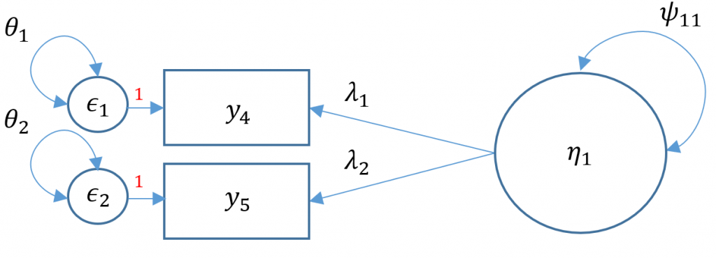
Technically a three item CFA is the minimum number of items for a one factor CFA as this results in a saturated model where the number of free parameters equals to number of elements in the variance-covariance matrix (i.e., the degrees of freedom is zero). Suppose that one of the data collectors accidentally lost part of the survey and we are left with only Items 4 and 5 from the SAQ-8. When there are only two items, you have $2(3)/2=3$ elements in the variance covariance matrix. As you can see in the path diagram below, there are in fact five free parameters: two residual variances $\theta_1, \theta_2$, two loadings $\lambda_1, \lambda_2$ and a factor variance $\psi_{11}$. Even if we used the marker method, which the default, that leaves us with one less parameter, $\lambda_1$ resulting in four free parameters when we only have three to work with.
If you simply ran the CFA mode as is you will get the following error
m2a <- 'f1 =~ q03 + q04' onefac2items <- cfa(m2a, data=dat) summary(onefac2items) <...output omitted ...> lavaan WARNING: Could not compute standard errors! The information matrix could not be inverted. This may be a symptom that the model is not identified.
The puzzle is to somehow fit a model that uses only three free parameters. One solution is to use the variance standardization method, which fixes the variance of the factor to one, and equate the second loading to equal the first loading. The gives us two residual variances $\theta_1, \theta_2$, and one loading to estimate $\lambda_1$. Can you think of other ways?
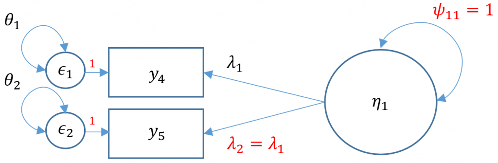
#one factor, two items (var std) m2b <- 'f1 =~ a*q04 + a*q05' onefac2items_b <- cfa(m2b, data=dat,std.lv=TRUE) summary(onefac2items_b) lavaan 0.6-5 ended normally after 8 iterations Estimator ML Optimization method NLMINB Number of free parameters 4 Number of equality constraints 1 Row rank of the constraints matrix 1 Number of observations 2571 Model Test User Model: Test statistic 0.000 Degrees of freedom 0 Parameter Estimates: Information Expected Information saturated (h1) model Structured Standard errors Standard Latent Variables: Estimate Std.Err z-value P(>|z|) f1 =~ q04 (a) 0.605 0.016 37.717 0.000 q05 (a) 0.605 0.016 37.717 0.000 Variances: Estimate Std.Err z-value P(>|z|) .q04 0.533 0.022 23.974 0.000 .q05 0.564 0.023 24.713 0.000 f1 1.000
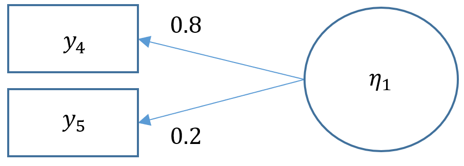
You can see from the output that although the total number of free parameters is four (two residual variances, two loadings), the degrees of freedom is zero because we have one equality constraint ($\lambda_2 = \lambda_1$). Note the (a) in front of the q04 Estimate means that we have attached a parameter label, and the additional (a) in front of the q05 means we have equated the two loadings, namely 0.605. The limitation of doing this is that there is no way to assess the fit of this model. For example, suppose we have the following hypothetical model where the true $\lambda_1=0.8$ and the true $\lambda_2=0.2$. If we fix $\lambda_1 = \lambda_2$, we would be able obtain a solution, not knowing that the model is a complete false representation of the truth since we cannot assess the fit of the model. It is always better to fit a CFA with more than three items and assess the fit of the model unless cost or theoretical limitations prevent you from doing otherwise.
One factor CFA with more than three items (SAQ-8)
The benefit of performing a one-factor CFA with more than three items is that a) your model is automatically identified because there will be more than 6 free parameters, and b) you model will not besaturatedmeaning you will have degrees of freedom left over to assess model fit.
To specify this lavaan, we again specify the model except we add Items 1 through 8 and store the object into m3a for Model 3A. Then pass this object into the wrapper function cfa and store the lavaan-method object into onefac8items but specify std.lv=TRUE to automatically use variance standardization. Finally, pass this object into summary but specify fit.measures=TRUE to obtain additional fit measures and standardized=TRUE to obtain both Std.lv and Std.all solutions.
#one factor eight items, variance std m3a <- 'f =~ q01 + q02 + q03 + q04 + q05 + q06 + q07 + q08' onefac8items_a <- cfa(m3a, data=dat,std.lv=TRUE) summary(onefac8items_a, fit.measures=TRUE, standardized=TRUE)
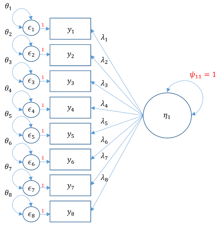
Model Test User Model: Test statistic 554.191 Degrees of freedom 20 P-value (Chi-square) 0.000 <... output omitted ...> Latent Variables: Estimate Std.Err z-value P(>|z|) Std.lv Std.all f =~ q01 0.485 0.017 28.942 0.000 0.485 0.586 q02 -0.198 0.019 -10.633 0.000 -0.198 -0.233 q03 -0.612 0.022 -27.989 0.000 -0.612 -0.570 q04 0.632 0.019 33.810 0.000 0.632 0.667 q05 0.554 0.020 28.259 0.000 0.554 0.574 q06 0.554 0.023 23.742 0.000 0.554 0.494 q07 0.716 0.022 32.761 0.000 0.716 0.650 q08 0.424 0.018 23.292 0.000 0.424 0.486
Looking at the Std.all loadings we see that Item 2 loads the weakest onto our SPSS Anxiety factor at -0.23 and Item 4 loads the highest at 0.67. Items 2 and 3 also load in a negative direction compared to the other items. You can see this clearly in the correlation table below, bolded values indicate bivariate corelations of Items 2 and 3 with all other items and all correlations are negative.
> round(cor(dat[,1:8]),2) q01 q02 q03 q04 q05 q06 q07 q08 q01 1.00 -0.10 -0.34 0.44 0.40 0.22 0.31 0.33 q02 -0.10 1.00 0.32 -0.11 -0.12 -0.07 -0.16 -0.05 q03 -0.34 0.32 1.00 -0.38 -0.31 -0.23 -0.38 -0.26 q04 0.44 -0.11 -0.38 1.00 0.40 0.28 0.41 0.35 q05 0.40 -0.12 -0.31 0.40 1.00 0.26 0.34 0.27 q06 0.22 -0.07 -0.23 0.28 0.26 1.00 0.51 0.22 q07 0.31 -0.16 -0.38 0.41 0.34 0.51 1.00 0.30 q08 0.33 -0.05 -0.26 0.35 0.27 0.22 0.30 1.0
Model Fit Statistics
For CFA models with more than three items, there is a way to assess how well the model fits the data, namely how close the (population) model-implied covariance matrix $\Sigma{(\theta)}$ matches the (population) observed covariance matrix $\Sigma$. The null and alternative hypotheses in a CFA model are
$$H_0: \Sigma{(\theta)}=\Sigma$$
$$H_1: \Sigma{(\theta)} \ne \Sigma$$
Typically, rejecting the null hypothesis is a good thing, but if we reject the CFA null hypothesis then we would reject our user model (which is bad). Failing to reject the model is good for our model because we have failed to disprove that our model is bad. Note that based on the logic of hypothesis testing, failing to reject the null hypothesis does not prove that our model is the true model, nor can we say it is the best model, as there may be many other competing models that can also fail to reject the null hypothesis. However, we can certainly say it it isn't a bad model, and it is the best model we can find at the moment. Think of a jury where it has failed to prove the criminal guilty, but it doesn't necessarily mean he is innocent. Can you think of a famous person from the 90's who fits this criteria?
Since we don't have the population covariances to evaluate, they are estimated by the sample model-implied covariance $\Sigma(\hat{\theta})$ and sample covariance $S$. Then the difference $S-\Sigma(\hat{\theta})$ is a proxy for the fit of the model, and is defined as the residual covariance with values close to zero indicating that there is a relatively good fit.
Quiz
T/F The residual covariance is defined as $\Sigma -\Sigma{(\theta)}$ and the closer this difference is to zero the better the fit.
Answer: False, the residual covariance uses sample estimates $S-\Sigma(\hat{\theta})$. Note that $\Sigma -\Sigma{(\theta)}=0$ is always true under the null hypothesis.
By default, lavaan outputs the model chi-square a.k.a Model Test User Model. To request additional fit statistics you add the fit.measures=TRUE option to summary, passing in the lavaan object onefac8items_a.
#fit statistics summary(onefac8items_a, fit.measures=TRUE, standardized=TRUE) lavaan 0.6-5 ended normally after 15 iterations Estimator ML Optimization method NLMINB Number of free parameters 16 Number of observations 2571 Model Test User Model: Test statistic 554.191 Degrees of freedom 20 P-value (Chi-square) 0.000 Model Test Baseline Model: Test statistic 4164.572 Degrees of freedom 28 P-value 0.000 User Model versus Baseline Model: Comparative Fit Index (CFI) 0.871 Tucker-Lewis Index (TLI) 0.819 Loglikelihood and Information Criteria: Loglikelihood user model (H0) -26629.559 Loglikelihood unrestricted model (H1) -26352.464 Akaike (AIC) 53291.118 Bayesian (BIC) 53384.751 Sample-size adjusted Bayesian (BIC) 53333.914 Root Mean Square Error of Approximation: RMSEA 0.102 90 Percent confidence interval - lower 0.095 90 Percent confidence interval - upper 0.109 P-value RMSEA <= 0.05 0.000 Standardized Root Mean Square Residual: SRMR 0.055
When fit measures are requested, lavaan outputs a plethora of statistics, but we will focus on the four commonly used ones:
- Model chi-square is the chi-square statistic we obtain from the maximum likelihood statistic (in lavaan, this is known as the Test Statistic for the Model Test User Model)
- CFI is the Comparative Fit Index – values can range between 0 and 1 (values greater than 0.90, conservatively 0.95 indicate good fit)
- TLI Tucker Lewis Index which also ranges between 0 and 1 (if it's greater than 1 it should be rounded to 1) with values greater than 0.90 indicating good fit. If the CFI and TLI are less than one, the CFI is always greater than the TLI.
- RMSEA is the root mean square error of approximation
- In
lavaan, you also obtain a p-value of close fit, that the RMSEA < 0.05. If you reject the model, it means your model is not a close fitting model.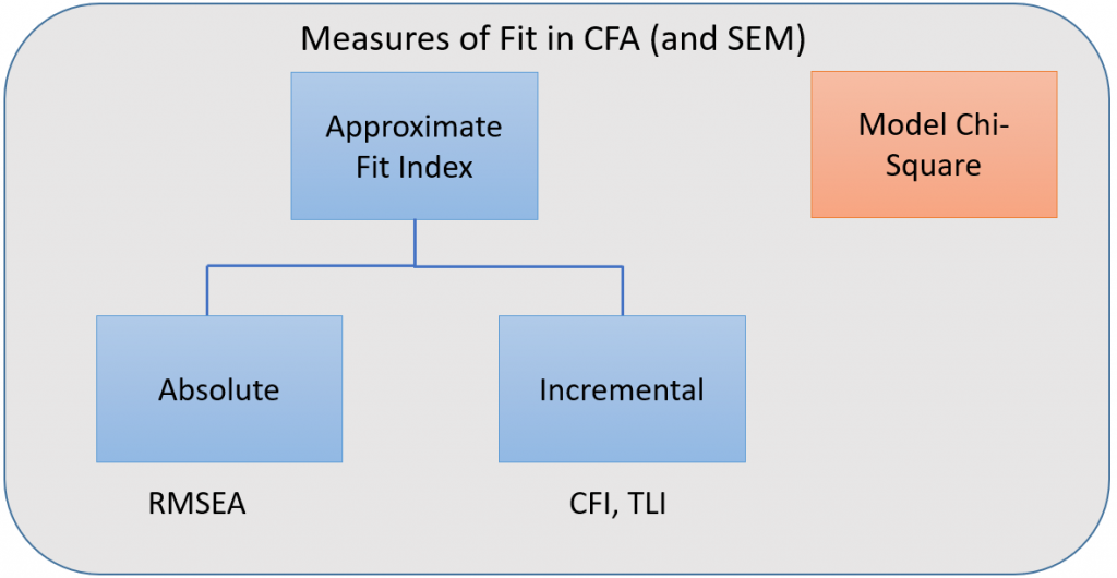
- In
Model chi-square
The model chi-square is defined as either $nF_{ML}$ or $(n-1)(F_{ML})$ depending on the statistical package where $n$ is the sample size and $F_{ML}$ is the fit function from maximum likelihood, which is a statistical method used to estimate the parameters in your model. The model chi-square is a meaningful test only when you have an over-identified model (i.e., there are still degrees of freedom left over after accounting for all the free parameters in your model).
The three-item CFA is saturated (meaning df=0) because we have $3(4)/2=6$ known values and 6 free parameters. For the eight-item model, we have 2o degrees of freedom.
Quiz
Explain how to obtain 20 degrees of freedom from the 8-item one factor CFA by first calculating the number of free parameters and comparing that to the number of known values.
Answer
First calculate the number of total parameters, which are 8 loadings $\lambda_1, \cdots, \lambda_8$, 8 residual variances $\theta_1, \cdots, \theta_8$ and 1 variance of the factor $\psi_{11}$. By the variance standardization method, we have fixed 1 parameter, namely $\psi_{11}=1$. The number of free parameters is then:
$$\mbox{no. free parameters} = 17 \mbox{ total parameters } – 1 \mbox{ fixed parameters } = 16.$$
Finally, there are $8(9)/2=36$ known values from the variance covariance matrix so the degrees of freedom is
$$\mbox{df} = 36 \mbox{ known values } – 16 \mbox{ free parameters} = 20.$$
Comparing the Model Test User Model for the eight-item (over-identified) model to the the three-item (saturated) model, we see that the Test Statistic degrees of freedom is zero for the three-item one factor CFA model indicating a saturated model, whereas the eight-item model has a positive degrees of freedom indicating an over-identified model. The Test Statistic is relatively large (554.191) and there is an additional row with P-value (Chi-square) indicating that we reject the null hypothesis.
#Three Item One-Factor CFA (Just Identified) Number of free parameters 6 Model Test User Model: Test statistic 0.000 Degrees of freedom 0 #Eight Item One-Factor CFA (Over-Identified) Number of free parameters 16 Model Test User Model: Test statistic 554.191 Degrees of freedom 20 P-value (Chi-square) 0.000
The larger the chi-square value the larger the difference between the sample implied covariance matrix $\Sigma{(\hat{\theta})}$ and the sample observed covariance matrix $S$, and the more likely you will reject your model. We can recreate the p-value which is essentially zero, using the density function of the chi-square with 20 degrees of freedom $\chi^2_{20}$. Note that scientific notation of $1.25 \times 10^{-104}$ means $125/10^{102}$ which is a really small number. Since $p < 0.05$, using the model chi-square criteria alone we reject the null hypothesis that the model fits the data. It is well documented in CFA and SEM literature that the chi-square is often overly sensitive in model testing especially for large samples. David Kenny states that for models with 75 to 200 cases chi-square is a reasonable measure of fit, but for 400 cases or more it is nearly almost always significant.
Quiz
T/F The larger the model chi-square test statistic, the larger the residual covariance.
Answer
True. Since the model chi-square is proportional to the discrepancy of $S$ and $\Sigma{(\hat{\theta})}$, the higher the chi-square the more positive the value of $S-\Sigma{(\hat{\theta})}$, defined as residual covariance.
Our sample of $n=2,571$ is considered relatively large, hence our conclusion may be supplemented with other fit indices.
#model chi-square > pchisq(q=554.191,df=20,lower.tail=FALSE) [1] 1.250667e-104
A note on sample size
Model chi-square is sensitive to large sample sizes, but does that mean we stick with small samples? The answer is no, larger samples are always preferred. CFA and the general class of structural equation model are actually large sample techniques and much of the theory is based on the premise that your sample size is as large as possible. So how big of a sample do we need? Kline (2016) notes the $N:q$ rule, which states that the sample size should be determined by the number of $q$ parameters in your model, and the recommended ratio is $20:1$. This means that if you have 10 parameters, you should have n=200. A sample size less than 100 is almost always untenable according to Kline.
(Optional) Model test of the baseline or null model
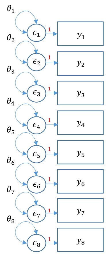
The model test baseline is also known as thenullmodel, where all covariances are set to zero and freely estimates variances. Rather than estimate the factor loadings, here we only estimate the observed means and variances (removing all the covariances). Recall that we have $p(p+1)/2$ covariances. Since we are only estimating the $p$ variances we have $p(p+1)/2-p$ degrees of freedom, or in this particular model $8(9)/2-8=28$ degrees of freedom. You can verify in the output below that we indeed have 8 free parameters and 28 degrees of freedom.
Think of the null or baseline model as the worst model you can come up with and the saturated model as the best model. Theoretically, the baseline model is useful for understanding how other fit indices are calculated.
#baseline b1 <- ' q01 ~~ q01 q02 ~~ q02 q03 ~~ q03 q04 ~~ q04 q05 ~~ q05 q06 ~~ q06 q07 ~~ q07 q08 ~~ q08' basemodel <- cfa(b1, data=dat) summary(basemodel) <... output ommitted ...> Number of free parameters 8 Model Test User Model: Test statistic 4164.572 Degrees of freedom 28 P-value (Chi-square) 0.000 Variances: Estimate Std.Err z-value P(>|z|) q01 0.685 0.019 35.854 0.000 q02 0.724 0.020 35.854 0.000 q03 1.155 0.032 35.854 0.000 q04 0.899 0.025 35.854 0.000 q05 0.930 0.026 35.854 0.000 q06 1.258 0.035 35.854 0.000 q07 1.215 0.034 35.854 0.000 q08 0.761 0.021 35.854 0.000
The figure below represents the same model above as a path diagram. Notice that the only parameters estimated are $\theta_1, \cdots, \theta_8$.
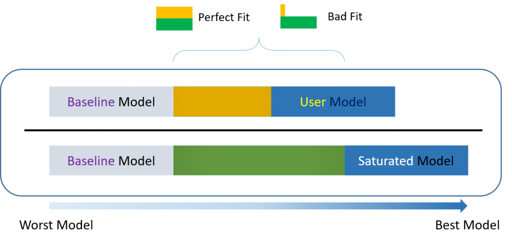
Incremental versus absolute fit index
For over-identified models, there are many types of fit indexes available to the researcher. Historically, model chi-square was the only measure of fit but in practice the null hypothesis was often rejected due to the chi-square's heightened sensitivity under large samples. To resolve this problem, approximate fit indexes that were not based on accepting or rejecting the null hypothesis were developed. Approximate fit indexes can be further classified into a) absolute and b) incremental or relative fit indexes. An incremental fit index(a.k.a. relative fit index) assesses the ratio of the deviation of the user model from the worst fitting model (a.k.a. the baseline model) against the deviation of the saturated model from the baseline model. Conceptually, if the deviation of the user model is the same as the deviation of the saturated model (a.k.a best fitting model), then the ratio should be 1. Alternatively, the more discrepant the two deviations, the closer the ratio is to 0 (see figure below). Examples of incremental fit indexes are the CFI and TLI. An absolute fit index on the other hand, does not compare the user model against a baseline model, but instead compares it to the observed data. An example of an absolute fit index is the RMSEA (see figure above).
CFI (Comparative Fit Index)
The CFI or comparative fit index is a popular fit index as a supplement to the model chi-square. Let $\delta=\chi^2 – df$ where $df$ is the degrees of freedom for that particular model. The closer $\delta$ is to zero, the more the model fits the data. The formula for the CFI is:
$$CFI= \frac{\delta(\mbox{Baseline}) – \delta(\mbox{User})}{\delta(\mbox{Baseline})} $$
To manually calculate the CFI, recall the selected output from the eight-item one factor model:
Model Test User Model: Test statistic 554.191 Degrees of freedom 20 P-value (Chi-square) 0.000 Model Test Baseline Model: Test statistic 4164.572 Degrees of freedom 28 P-value 0.000
Then $\chi^2(\mbox{Baseline}) = 4164.572$ and $df({\mbox{Baseline}}) = 28$, and $\chi^2(\mbox{User}) = 554.191$ and $df(\mbox{User}) = 20$. So $\delta(\mbox{Baseline}) = 4164.572 – 28 =4136.572$ and $\delta(\mbox{User} )= 554.191 – 20=534.191$. We can plug all of this into the following equation:
$$CFI= \frac{4136.572- 534.191}{4136.572}=\frac{3602.381}{4136.572}=0.871$$
If $\delta(\mbox{User})=0$, then it means that the user model is not misspecified, so the numerator becomes $\delta(\mbox{Baseline})$ and the ratio becomes 1. The closer the CFI is to 1, the better the fit of the model; with the maximum being 1. Some criteria claims 0.90 to 0.95 as a good cutoff for good fit [citation needed].
TLI (Tucker Lewis Index)
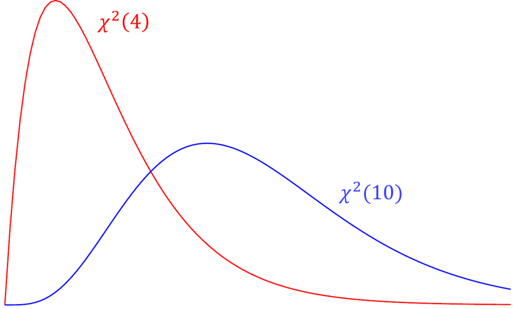
The Tucker Lewis Index is also an incremental fit index that is commonly outputted with the CFI in popular packages such as Mplus and in this case lavaan. The term used in the TFI is the relative chi-square (a.k.a. normed chi-square) defined as $\frac{\chi^2}{df}$. Compared to the model chi-square, relative chi-square is less sensitive to sample size. To understand relative chi-square, we need to know that the expected value or mean of a chi-square is its degrees of freedom (i.e., $E(\chi^2(df)) = df$). For example, given that the test statistic truly came from a chi-square distribution with 4 degrees of freedom, we would expect the average chi-square value across repeated samples would also be 4. Suppose the chi-square from our data actually came from a distribution with 10 degrees of freedom but our model says it came from a chi-square with 4 degrees of freedom. Over repeated sampling, the relative chi-square would be $10/4=2.5$. Thus, $\chi^2/df = 1$ indicates perfect fit, and some researchers say that a relative chi-square greater than 2 indicates poor fit (Byrne,1989), other researchers recommend using a ratio as low as 2 or as high as 5 to indicate a reasonable fit (Marsh and Hocevar, 1985).
Quiz
Suppose you ran a CFA with 20 degrees of freedom. What would be the acceptable range of chi-square values based on the criteria that the relative chi-square greater than 2 indicates poor fit?
Answer
The range of acceptable chi-square values ranges between 20 (indicating perfect fit) and 40, since 40/20 = 2.
The TLI is defined as
$$TLI= \frac{\mbox{min}(\chi^2(\mbox{Baseline})/df(\mbox{Baseline}),1)-\mbox{min}(\chi^2(\mbox{User})/df(\mbox{User}),1)}{\mbox{min}(\chi^2(\mbox{Baseline})/df(\mbox{Baseline}),1)-1}$$
In the denominator we have a 1 since $\chi^2(\mbox{Saturated})=0$ and $df(\mbox{Saturated})=0$ implies that $\mbox{min}(\chi^2(\mbox{Saturated})/df(\mbox{Saturated}),1)=1$. Also, the TLI can be greater than 1 but for practical purposes we round it to 1. Given the eight-item one factor model:
$$TLI= \frac{4164.572/28-554.191/20}{4164.572/28-1} =0.819.$$
We can confirm our answers for both the TLI and CFI which are reported together in lavaan
User Model versus Baseline Model: Comparative Fit Index (CFI) 0.871 Tucker-Lewis Index (TLI) 0.819
You can think of the TLI as the ratio of the deviation of the null (baseline) model from user model to the deviation of the baseline (or null) model to the perfect fit model $\chi^2/df = 1$. The more similar the deviation from the baseline model, the closer the ratio to one. A perfect fitting model which generate a TLI which equals 1. David Kenny states that if the CFI is less than one, then the CFI is always greater than the TLI. CFI pays a penalty of one for every parameter estimated. Because the TLI and CFI are highly correlated, only one of the two should be reported.
RMSEA
The root mean square error of approximation is an absolute measure of fit because it does not compare the discrepancy of the user model relative to a baseline model like the CFI or TLI. Instead, RMSEA defines $\delta$ as the non-centrality parameter which measures the degree of misspecification. Recall from the CFI that $\delta=\chi^2 – df$ where $df$ is the degrees of freedom for that particular model. The greater the $\delta$ the more misspecified the model.
$$ RMSEA = \sqrt{\frac{\delta}{df(n-1)}} $$
where $n$ is the total number of observations. The cutoff criteria as defined in Kline (2016, p.274-275)
- $\le 0.05$ (close-fit)
- between $.05$ and $.08$ (reasonable approximate fit, fails close-fit but also fails poor-fit)
- $>= 0.10$ (poor-fit)
In the case of our SAQ-8 factor analysis, $n=2,571$, $df(\mbox{User}) = 20$ and $\delta(\mbox{User} )= 534.191$ which we already known from calculating the CFI. Here $\delta$ is large relative to degrees of freedom.
$$ RMSEA = \sqrt{\frac{534.191}{20(2570)}} = \sqrt{0.0104}=0.102$$
Our RMSEA = 0.10 indicating poor fit, as evidence by the large $\delta(\mbox{User} )$ relative to the degrees of freedom.
Number of observations 2571 <... output omitted ...> Root Mean Square Error of Approximation: RMSEA 0.102 90 Percent confidence interval - lower 0.095 90 Percent confidence interval - upper 0.109 P-value RMSEA <= 0.05 0.000
Given that the p-value of the model chi-square was less than 0.05, the CFI = 0.871 and the RMSEA = 0.102, and looking at the standardized loadings we report to the Principal Investigator that the SAQ-8 as it stands does not possess good psychometric properties. Perhaps SPSS Anxiety is a more complex measure that we first assume.
Two Factor Confirmatory Factor Analysis
Although the results from the one-factor CFA suggest that a one factor solution may capture much of the variance in these items, the model fit suggests that this model can be improved. From the exploratory factor analysis, we found that Items 6 and 7 "hang" together. Let's take a look at Items 6 and 7 more carefully.
- Item 6: My friends are better at statistics than me
- Item 7: All computers hate me
Additionally, from the previous CFA we found that the Item 2 loaded poorly with the other items, with a standardized loading of only -0.23. From talking to the Principal Investigator, we decide the use only Items 1, 3, 4, 5, and 8 as indicators of SPSS Anxiety and Items 6 and 7 as indicators of Attribution Bias.
Uncorrelated factors
We will now proceed with a two-factor CFA where we assume uncorrelated (or orthogonal) factors. Having a two-item factor presents a special problem for identification. In order to identify a two-item factor there are two options:
- Freely estimate the loadings of the two items on the same factor but equate them to be equal while setting the variance of the factor at 1
- Freely estimate the variance of the factor, using the marker method for the first item, but covary (correlate) the two-item factor with another factor
Since we are doing an uncorrelated two-factor solution here, we are relegated to the first option.
#uncorrelated two factor solution, var std method m4a <- 'f1 =~ q01+ q03 + q04 + q05 + q08 f2 =~ a*q06 + a*q07 f1 ~~ 0*f2 ' twofac7items_a <- cfa(m4a, data=dat,std.lv=TRUE) #alternative syntax - uncorrelated two factor solution, var std method twofac7items_a <- cfa(m4a, data=dat,std.lv=TRUE, auto.cov.lv.x=FALSE) summary(twofac7items_a, fit.measures=TRUE,standardized=TRUE)
Since we have 7 items, the total elements in our variance covariance matrix is $7(8)/2=28$. The number of free parameters to be estimated include 7 residual variances $\theta_1, \cdots, \theta_7$, 7 loadings $\lambda_1, \cdots, \lambda_7$ for a total of 14. Then we have $28-14=14$ degrees of freedom. However for identification of the two indicator factor model, we constrained the loadings of Item 6 and Item 7 to be equal, which frees up a parameter and hence we end up with $14+1=15$ degrees of freedom.
lavaan 0.6-7 ended normally after 14 iterations Estimator ML Optimization method NLMINB Number of free parameters 14 Number of equality constraints 1 Number of observations 2571 Model Test User Model: Test statistic 841.205 Degrees of freedom 15 P-value (Chi-square) 0.000 Model Test Baseline Model: Test statistic 3876.345 Degrees of freedom 21 P-value 0.000 User Model versus Baseline Model: Comparative Fit Index (CFI) 0.786 Tucker-Lewis Index (TLI) 0.700 Loglikelihood and Information Criteria: Loglikelihood user model (H0) -23684.164 Loglikelihood unrestricted model (H1) -23263.562 Akaike (AIC) 47394.328 Bayesian (BIC) 47470.405 Sample-size adjusted Bayesian (BIC) 47429.101 Root Mean Square Error of Approximation: RMSEA 0.146 90 Percent confidence interval - lower 0.138 90 Percent confidence interval - upper 0.155 P-value RMSEA <= 0.05 0.000 Standardized Root Mean Square Residual: SRMR 0.180 Parameter Estimates: Standard errors Standard Information Expected Information saturated (h1) model Structured Latent Variables: Estimate Std.Err z-value P(>|z|) Std.lv Std.all f1 =~ q01 0.539 0.017 31.135 0.000 0.539 0.651 q03 -0.573 0.023 -24.902 0.000 -0.573 -0.533 q04 0.652 0.020 33.032 0.000 0.652 0.687 q05 0.567 0.020 27.812 0.000 0.567 0.588 q08 0.431 0.019 22.862 0.000 0.431 0.494 f2 =~ q06 (a) 0.797 0.017 46.329 0.000 0.797 0.710 q07 (a) 0.797 0.017 46.329 0.000 0.797 0.723 Covariances: Estimate Std.Err z-value P(>|z|) Std.lv Std.all f1 ~~ f2 0.000 0.000 0.000 Variances: Estimate Std.Err z-value P(>|z|) Std.lv Std.all .q01 0.395 0.015 26.280 0.000 0.395 0.576 .q03 0.827 0.027 30.787 0.000 0.827 0.716 .q04 0.474 0.020 24.230 0.000 0.474 0.527 .q05 0.608 0.021 29.043 0.000 0.608 0.654 .q08 0.575 0.018 31.760 0.000 0.575 0.756 .q06 0.623 0.027 22.916 0.000 0.623 0.495 .q07 0.580 0.026 21.925 0.000 0.580 0.477 f1 1.000 1.000 1.000 f2 1.000 1.000 1.000
Here's what the model looks like graphically:
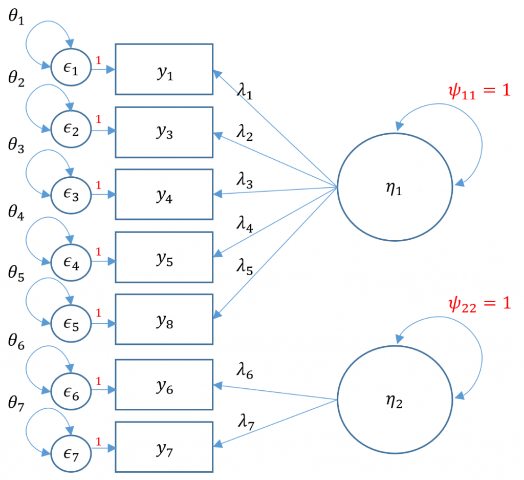
Since we picked Option 1, we set the loadings to be equal to each other:
f2 =~ q06 (a) 0.797 0.017 46.329 0.000 0.797 0.710 q07 (a) 0.797 0.017 46.329 0.000 0.797 0.723
We know the factors are uncorrelated because the estimate of f1 ~~ f2 is zero under the Covariances, which is what we expect.
Covariances: Estimate Std.Err z-value P(>|z|) Std.lv Std.all f1 ~~ f2 0.000 0.000 0.000
Looking at the model fit
Model Test User Model: Test statistic 841.205 Degrees of freedom 15 P-value (Chi-square) 0.000 User Model versus Baseline Model: Comparative Fit Index (CFI) 0.786 Tucker-Lewis Index (TLI) 0.700 Root Mean Square Error of Approximation: RMSEA 0.146 90 Percent confidence interval - lower 0.138 90 Percent confidence interval - upper 0.155 P-value RMSEA <= 0.05 0.000
We can see that the uncorrelated two factor CFA solution gives us a higher chi-square (lower is better), higher RMSEA and lower CFI/TLI, which means overall it's a poorer fitting model. We talk to the Principal Investigator and decide to go with a correlated (oblique) two factor model.
Correlated factors
We proceed with a correlated two-factor CFA. We still have the issue of that two-item factor; recall that for identification we can either equate the loadings and set the variance to 1 or we can covary the two-item factor with another factor and use the marker method. Taking advantage of our correlated factors, let's use the second option.
#correlated two factor solution, marker method m4b <- 'f1 =~ q01+ q03 + q04 + q05 + q08 f2 =~ q06 + q07' twofac7items_b <- cfa(m4b, data=dat,std.lv=TRUE) summary(twofac7items_b,fit.measures=TRUE,standardized=TRUE)
Although lavaan defaults to the marker method, by specifyingstandardized=TRUE we then implement the variance standardization method.
lavaan 0.6-7 ended normally after 18 iterations Estimator ML Optimization method NLMINB Number of free parameters 15 Number of observations 2571 Model Test User Model: Test statistic 66.768 Degrees of freedom 13 P-value (Chi-square) 0.000 Model Test Baseline Model: Test statistic 3876.345 Degrees of freedom 21 P-value 0.000 User Model versus Baseline Model: Comparative Fit Index (CFI) 0.986 Tucker-Lewis Index (TLI) 0.977 Loglikelihood and Information Criteria: Loglikelihood user model (H0) -23296.945 Loglikelihood unrestricted model (H1) -23263.562 Akaike (AIC) 46623.891 Bayesian (BIC) 46711.672 Sample-size adjusted Bayesian (BIC) 46664.013 Root Mean Square Error of Approximation: RMSEA 0.040 90 Percent confidence interval - lower 0.031 90 Percent confidence interval - upper 0.050 P-value RMSEA <= 0.05 0.952 Standardized Root Mean Square Residual: SRMR 0.021 Parameter Estimates: Standard errors Standard Information Expected Information saturated (h1) model Structured Latent Variables: Estimate Std.Err z-value P(>|z|) Std.lv Std.all f1 =~ q01 0.513 0.017 30.460 0.000 0.513 0.619 q03 -0.599 0.022 -26.941 0.000 -0.599 -0.557 q04 0.658 0.019 34.876 0.000 0.658 0.694 q05 0.567 0.020 28.676 0.000 0.567 0.588 q08 0.435 0.018 23.701 0.000 0.435 0.498 f2 =~ q06 0.669 0.025 27.001 0.000 0.669 0.596 q07 0.949 0.027 35.310 0.000 0.949 0.861 Covariances: Estimate Std.Err z-value P(>|z|) Std.lv Std.all f1 ~~ f2 0.676 0.020 33.023 0.000 0.676 0.676 Variances: Estimate Std.Err z-value P(>|z|) Std.lv Std.all .q01 0.423 0.014 29.157 0.000 0.423 0.617 .q03 0.796 0.026 31.025 0.000 0.796 0.689 .q04 0.466 0.018 25.824 0.000 0.466 0.518 .q05 0.608 0.020 30.173 0.000 0.608 0.654 .q08 0.572 0.018 32.332 0.000 0.572 0.752 .q06 0.811 0.030 27.187 0.000 0.811 0.644 .q07 0.314 0.040 7.815 0.000 0.314 0.258 f1 1.000 1.000 1.000 f2 1.000 1.000 1.000
Notice that compared to the uncorrelated two-factor solution, the chi-square and RMSEA are both lower. The test of RMSEA is not significant which means that we do not reject the null hypothesis that the RMSEA is less than or equal to 0.05. Additionally the CFI and TLI are both higher and pass the 0.95 threshold. This is even better fitting than the one-factor solution. After talking with the Principal Investigator, we choose the final two correlated factor CFA model as shown below.
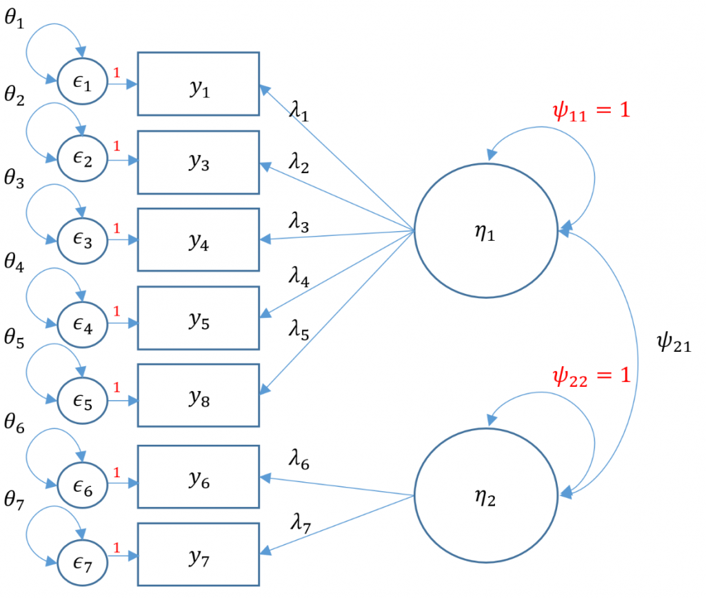
Since we have 7 items, the total elements in our variance covariance matrix is $7(8)/2=28$. The number of free parameters to be estimated include 7 residual variances $\theta_1, \cdots, \theta_7$, 7 loadings $\lambda_1, \cdots, \lambda_7$ one covariance $\psi_{21}$ for a total of 15. Then $28-15=13$ degrees of freedom.
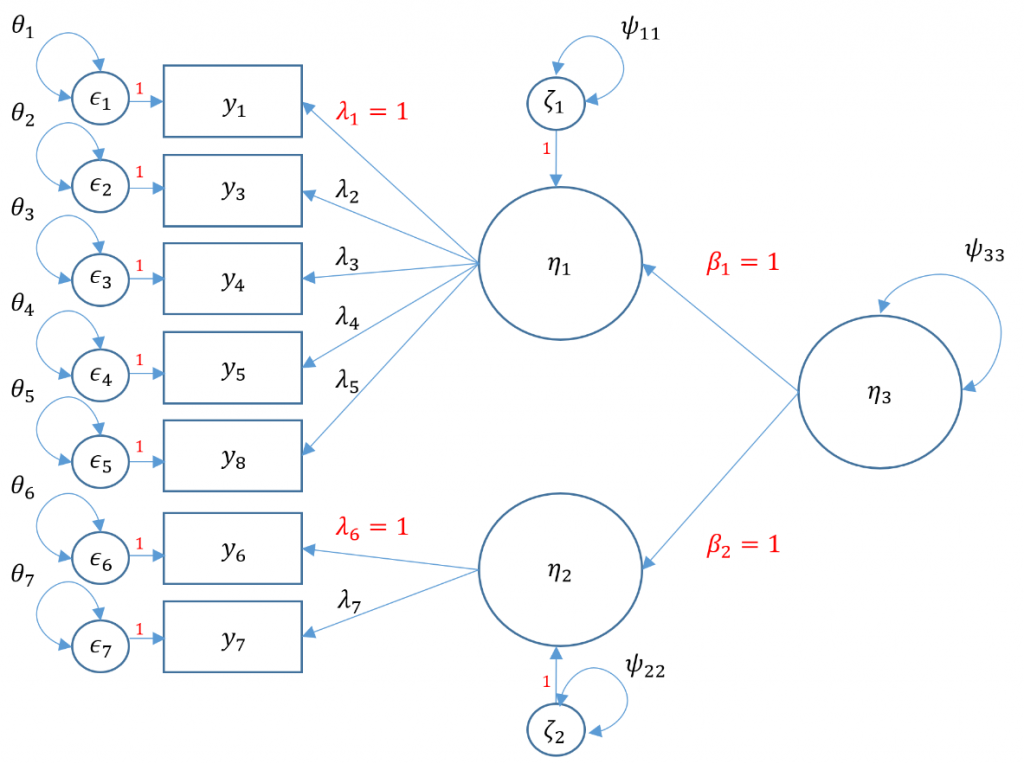
Second-Order CFA
Suppose the Principal Investigator believes that the correlation between SPSS Anxiety and Attribution Bias are first-order factors is caused more by the second-order factor, overall Anxiety. In order to undrestand the model, we have to understand endogenousandexogenousfactors. In simple terms, an endogenous factor is a factor that is being predicted by another factor (or variable in general), and an exogenous factor is a factor that is not being predicted by another. The main difference is that endogenous factors now have a residual variance as it is not being predicted by another latent variable known as $\zeta$. The residual variance is essentially the variance of $\zeta$, which we classify here as $\psi$.
To calculate the total number of free parameters, again there are seven items so there are $7(8)/2=28$ elements in the variance covariance matrix. Identification of a second order factor is the same process as identification of a single factor except you treat the first order factor as indicators rather than as observed outcomes. The only main difference is that instead of an observed residual variance $\theta$, the residual variance of a factor is classified under the $\Psi$ matrix. Without going into the technical details (see optional section), you can think of the factor residual variance as another variance parameter. There are seven residual variances $\theta_1, \cdots, \theta_7$, seven loadings $\lambda_1, \cdots \lambda_7$. Additionally, since we have two endogenous factors which have their own residual variances $\psi_{11}, \psi_{22}$
#second order three factor solution, marker method m5a <- 'f1 =~ q01+ q03 + q04 + q05 + q08 f2 =~ q06 + q07 f3 =~ 1*f1 + 1*f2 f3 ~~ f3' secondorder <- cfa(m5a, data=dat) summary(secondorder,fit.measures=TRUE,standardized=TRUE) lavaan 0.6-5 ended normally after 30 iterations Estimator ML Optimization method NLMINB Number of free parameters 15 Number of observations 2571 Model Test User Model: Test statistic 66.768 Degrees of freedom 13 P-value (Chi-square) 0.000 Model Test Baseline Model: Test statistic 3876.345 Degrees of freedom 21 P-value 0.000 User Model versus Baseline Model: Comparative Fit Index (CFI) 0.986 Tucker-Lewis Index (TLI) 0.977 Loglikelihood and Information Criteria: Loglikelihood user model (H0) -23296.945 Loglikelihood unrestricted model (H1) -23263.562 Akaike (AIC) 46623.891 Bayesian (BIC) 46711.672 Sample-size adjusted Bayesian (BIC) 46664.013 Standardized Root Mean Square Residual: SRMR 0.021 Parameter Estimates: Information Expected Information saturated (h1) model Structured Standard errors Standard Latent Variables: Estimate Std.Err z-value P(>|z|) Std.lv Std.all f1 =~ q01 1.000 0.513 0.619 q03 -1.169 0.054 -21.714 0.000 -0.599 -0.557 q04 1.284 0.051 25.011 0.000 0.658 0.694 q05 1.107 0.049 22.572 0.000 0.567 0.588 q08 0.848 0.043 19.927 0.000 0.435 0.498 f2 =~ q06 1.000 0.669 0.596 q07 1.419 0.071 20.065 0.000 0.949 0.861 f3 =~ f1 1.000 0.939 0.939 f2 1.000 0.720 0.720 Variances: Estimate Std.Err z-value P(>|z|) Std.lv Std.all f3 0.232 0.015 15.175 0.000 1.000 1.000 .q01 0.423 0.014 29.157 0.000 0.423 0.617 .q03 0.796 0.026 31.025 0.000 0.796 0.689 .q04 0.466 0.018 25.824 0.000 0.466 0.518 .q05 0.608 0.020 30.173 0.000 0.608 0.654 .q08 0.572 0.018 32.332 0.000 0.572 0.752 .q06 0.811 0.030 27.187 0.000 0.811 0.644 .q07 0.314 0.040 7.815 0.000 0.314 0.258 .f1 0.031 0.015 2.057 0.040 0.118 0.118 .f2 0.216 0.024 8.867 0.000 0.482 0.482
Note that there is no perfect way to specify a second order factor when you only have two first order factors. You either have to assume The variance standardization method assumes that the residual variance of the two first order factors is one which means that you assume homogeneous residual variance. The marker method assumes that both loadings from the second order factor to the first factor is 1. To make sure you fit an equivalent method though, the degrees of freedom for the User model must be the same. NOTE: changing the standardization method should not change the degrees of freedom and chi-square value. If you standardize it one way and get a different degrees of freedom, then you have identified it incorrectly. Even though the chi-square fit is the same however, you will get different standardized variances and loadings depending on the the assumptions you make (to set the loadings to 1 for the two first order factors and freely estimate the variance or to freely estimate but equate the loadings and set the residual variance of the first order factors to 1).
(Optional) Warning message with second-order CFA
The warning message is an indication that your model is not identified rather than a problem with the data.
Warning message: In lav_model_vcov(lavmodel = lavmodel2, lavsamplestats = lavsamplestats, : lavaan WARNING: The variance-covariance matrix of the estimated parameters (vcov) does not appear to be positive definite! The smallest eigenvalue (= 2.211069e-19) is close to zero. This may be a symptom that the model is not identified.
Note the following marker method below is the correct identification. The syntax NA*f1 means to free the first loading because by default the marker method fixes the loading to 1, and equal("f3=~f1")*f2 fixes the loading of the second factor on the third to be the same as the first factor.
#second order three factor solution, var std method m5b <- 'f1 =~ NA*q01+ q03 + q04 + q05 + q08 f2 =~ NA*q06 + q07 f3 =~ NA*f1 + equal("f3=~f1")*f2 f1 ~~ 1*f1 f2 ~~ 1*f2 f3 ~~ 1*f3' secondorder <- cfa(m5b, data=dat) summary(secondorder,fit.measures=TRUE) <...output omitted ...> Model Test User Model: Test statistic 66.768 Degrees of freedom 13 P-value (Chi-square) 0.000 (Optional) Obtaining the parameter table
To see internally how lavaan stores the parameters, you can inspect your model output and request a partable or parameter table. For users of LISREL, you will notice that lavaan sticks with Y-side matrix notation (i.e., no differentiation is made between exogenous and endogenous latent variables). For example, typical $\phi$ variance and covariances parameters for exogenous latent variables will be incorporated into the $\Psi$ matrix which in full LISREL notation is reserved for variance and covariances parameters for endogenous latent variables.
#obtain the parameter table of the second order factor > inspect(secondorder,"partable") Note: model contains equality constraints: lhs op rhs 1 6 == 7 2 8 == 9 $lambda f1 f2 f3 q01 1 0 0 q03 2 0 0 q04 3 0 0 q05 4 0 0 q08 5 0 0 q06 0 6 0 q07 0 7 0 $theta q01 q03 q04 q05 q08 q06 q07 q01 13 q03 0 14 q04 0 0 15 q05 0 0 0 16 q08 0 0 0 0 17 q06 0 0 0 0 0 18 q07 0 0 0 0 0 0 19 $psi f1 f2 f3 f1 10 f2 0 11 f3 0 0 12 $beta f1 f2 f3 f1 0 0 8 f2 0 0 9 f3 0 0 0
Conclusion
CFA distinguishes itself from EFA as a method to assess the credibility of a previously defined hypothesis, namely that the model implied covariance matrix $\Sigma(\Theta)$ as defined by the measurement model, can faithfully reproduce the observed covariance matrix $\Sigma$. Suppose you find that SPSS Anxiety can be adequately represented by the first eight items in your scale, you fail to reject the null hypothesis and therefore your chi-square is significant. However, if the chi-square is significant, it may be possible that the rejection is due to the sensitivity of the chi-square to large samples rather than a true rejection of the model. Therefore, it its place often times researchers use fit index criteria such as the CFI > 0.95, TLI > 0.90 and RMSEA < 0.10 to support their claim. Due to its goal of reproducing the observed covariance matrix, its free parameters are completely determined by the dimensions of $\Sigma$. As such, identification is a key method of ensuring that the number of free parameters is less than or equal to the total number of parameters, by instilling fixed parameters. The observed indicators serve as measures of the unobserved construct or factor. A just identified model for a one-factor model has exactly three indicators, but some researchers require only two indicators per factor due to resource restrictions; however having more than three items per factor is ideal because it allows degrees of freedom which leads to measures of fit. Finally, if the fit indicates poor fit for a one-factor model, a two-factor model may be more appropriate, that the items measure not just one construct, and that there may be underlying correlation between the two constructors or factor. However, if theory is that the correlation between these two constructs is caused by a third factor, then these two first-order factors can serve as latent indicators of the underlying second order factor. However if the correlations between factors are represented as regression paths, then we move beyond the scope of this seminar into what is known as structural equation modeling. We hope you have found this introductory seminar to be useful, and we wish you best of luck on your research endeavors.
Appendix
For those readers who are more mathematically inclined, the appendix adds additional details.
Assumptions of the factor analysis model
In traditional confirmatory factor analysis or structural equation modeling, the
- mean of the intercepts is zero \(E(\tau)=0\) (not tenable, this is no longer true with modern full information CFA/SEM, see Kline 2016)
- mean of the factor is zero \(E(\eta)=0\)
- mean of the residual is zero \(E(\epsilon)=0\)
- covariance of the factor with the residual is zero \(Cov(\eta,\epsilon)=0\)
These simplified assumptions can help us calculate the expectation and the variance of the multivariate outcome $\mathbf{y}$:
Expectation
$$ \begin{eqnarray} \mathbf{\mu_y} = E(\mathbf{y}) &=& E(\mathbf{\tau} + \mathbf{\Lambda} \mathbf{\eta} + \mathbf{\epsilon}) \\ &=& E(\mathbf{\tau} )+E( \mathbf{\Lambda} \mathbf{\eta}) + E(\mathbf{\epsilon}) \\ &=& 0 + E( \mathbf{\Lambda} \mathbf{\eta}) + 0 \\ &=& E( \mathbf{\Lambda} \mathbf{\eta}) \\ &=& \mathbf{\Lambda} E(\mathbf{\eta}) \\ &=& \mathbf{\Lambda} \mathbf{\eta} \end{eqnarray} $$
This is due to the assumptions from above and properties of expectation.
Covariance structure
$$ \begin{eqnarray} \Sigma(\theta) = Cov(\mathbf{y}) & = & Cov(\mathbf{\tau} + \mathbf{\Lambda} \mathbf{\eta} + \mathbf{\epsilon}) \\ & = & Var(\mathbf{\tau}) + Cov(\mathbf{\Lambda} \mathbf{\eta}) + Var(\mathbf{\epsilon}) \\ & = & 0 + Cov(\mathbf{\Lambda} \mathbf{\eta}) + Var(\mathbf{\epsilon}) \\ & = & \mathbf{\Lambda} Cov(\mathbf{\eta}) \mathbf{\Lambda}' + Var(\mathbf{\epsilon}) \\ & = & \mathbf{\Lambda} \Psi \mathbf{\Lambda}' + \Theta_{\epsilon} \\ \end{eqnarray} $$
This is true due to the assumptions we made above and properties of covariance, such as the fact that the variance of a constant is zero and \(Cov(AB)=A Cov(B) A'\). We have defined new matrices where \(Cov(\mathbf{\eta}) = \Psi\) is the variance-covariance matrix of the factors \(\eta\) and \(Var(\mathbf{\epsilon})=\Theta_{\epsilon}\) is the variance of the residuals.
References
For more information on:
- lavaan's own tutorial http://lavaan.ugent.be/tutorial
- extracting objects from lavaan Inspect or extract information from a fitted lavaan object
Saturated versus baseline models
- What are the saturated and baseline models in sem?
- Google Forums
- Disentangling degrees of freedom
Fit indexes
- Research Gate Discussion about Chi-Square
- Assess whole SEM model–chi square and fit index
Source: https://stats.idre.ucla.edu/r/seminars/rcfa/
Posted by: badrenovieren02.blogspot.com